What is This About?
Not to be confused with analysis of variance (ANOVA), variance analysis or budget variance analysis is a staple of management accounting.
It is the process used to compare a budgeted metric with the actual incurred metric.
In this post, we will go over a quick review of variance analysis and then introduce the first one of a long series of improvements needed to achieve a more accurate depiction of financial reality.
Quick Review
Please, feel free to skip this section if you are already familiar with the concept.
Before diving in, I would like to ask you a question!
How do you assess your performance when you go shopping?
You compare how much you had expected to spend with how much you actually spent?
If we note our expenditures X, our performance could be quantified like this:

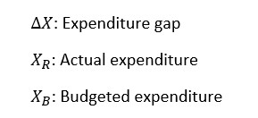
Here is the meaning of the notation:

This might be enough if you were only worried about exceeding your budget.
However, it doesn not tell us much about the actual explanation of the performance.
We would like to dig one level deeper to see how this performance is formed.
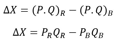
We can start with the realization that expenditure is the product of price and quantity:

We can express our expenditure gap as follows:

If we introduce gaps in quantity and price in the formula, we get:


We can then simplify and rearrange the items in the formula to ease interpretation:

Our expenditure gap can be expressed as the sum of a quantity effect (QE) and a price effect (PE).
This can help us further dissect our performance: how much did we gain or lose through each effect? are the effects reinforcing each other or do they nullify each other?
In many cases, this can also help us improve the forecasting system itself, as systematically negative effects would indicate a biais in the predictive model.
In practice this can be done for any metric that is the product of two variables: cost of materials, cost of labor, sales, change in inventory etc.
But why stop here?
Generalization to N Variables
As the French say: “jamais deux sans trois”.
We can throw in a third variable for fun.
Suppose all our sales are foreign (we will conveniently ignore all the irrelevant issues such as currency of reporting).
We would need to account for the currency exchange rate (denoted C).
In this case our sales (in domestic currency) would be the product of three variables:

Quick algebra allows us to derive the following menacing equation:

A clear trend seems to emerge in this equation as we increase the number of variables.
First, we get N distinct effects to explain our total variance.
Second, we change one variable at a time while keeping others constant (relative to the last effect computed).
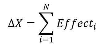
Our total variance can thus be entirely explained with the following formula:

This is what I would call the multiplication paradigm.
You explain total variance by deconstructing your metric into a product of variables.
It does a decent job at approximating reality.
However, if you play with it long enough, you will notice something is wrong.
The Implicit Assumption
Before we address the issue, it might be helpful to reframe what we have done so far.
Yes, we are looking to evaluate performance but more accurately we are splitting our total variance into “independent” explaining factors.
The total variance is unchanged, it is a given.
It follows that an underestimated effect will lead to one or several other overestimated effects.
This is why it is important to get each effect right.
Now to address the issue, consider the following case study.
Metaverse Land Case Study
We are a software company and we sell imaginary pieces of land in the metaverse.
We charge not-so-imaginary US dollars for each purchase.
Our pieces of land can be either building land or unbuildable land.
We expected the following breakdown for our sales (in surface area units): 70% building land and 30% unbuildable land.
After the annual closing, our sales mix turned out to be: 80% building land and 20% unbuildable land.
The breakdown of our total sales is as follows:
- Expected (average) price: $85
- Actual (average) price: $96
- Expected volume: 30,000m²
- Actual volume: 50,000m²
We decide out of curiosity to separately analyze each of our sales segments:
Building land:
- Expected price: $100
- Actual price: $110
- Expected volume: 21,000m²
- Actual volume: 40,000m²
- Expected % of sales (in m²): 70%
- Actual % of sales: 80%
Unbuildable land:
- Expected price: $50
- Actual price: $40
- Expected volume: 9,000m²
- Actual volume: 10,000m²
- Expected % of sales (in m²): 30%
- Actual % of sales: 20%
Let’s compute the total variance and the explaining effects for each type of land and for the total:
Total land:
- Total variance: $2.25M
- Quantity effect: $1.7M
- Price effect: $0.55M
Building land:
- Total variance: $2.3M
- Quantity effect: $1.9M
- Price effect: $0.4M
Unbuildable land:
- Total variance: -$0.05M
- Quantity effect: $0.05M
- Price effect: -$0.1M
You will get a surprising result when you sum up the individual price effects and compare them with the price effect of the total land.
It is overestimated by $0.25M in our total land calculations.
Naturally, this gap shows up with the opposite sign when we do the same exercise for the quantity effect.
The total variance is unaffected however, taken as a whole or as the sum of the segments.
You can download the case study (in an Excel file) by following this link:
This case study highlights one of the biggest flaws of variance analysis taken at face value.
It assumes your metric follows a constant linear underlying structure.
In other words, as long your sales mix stays the same, you should be fine.
This case study might seem contrived with its arbitrary round numbers.
However, change is the norm in nature and you should be wondering why your mix would rather stay the same than fluctuate.
If only for differentials in inflation, any mix could be subject to change at some point.
Resolution and Image Quality
More importantly, there is a stronger reason to address this issue.
Business units are often very complex with many product lines and arbitrary subdivisions such as geography, demographics, designs, specifications…
Each one of these variables might alter the balance between price and quantity effects.
These differences can add up to a meaningful amount at the scale of a firm.
Especially over longer periods of time when the metric’s underlying mix might drift.
Worse, this issue could affect all the metrics followed by the company with variance analysis: sales, change in inventories, COGS etc.
Furthermore, a low-resolution snapshot can induce management into error as it may hide many realities and lend itself to faulty interpretations.
The best and worst scenarios that can be derived from this low-resolution snapshot can be very different (leading to possibly contradictory decisions).

(Image: @Chicken3gg/Twitter)

(Image: @Chicken3gg/Twitter)
This is why it is of utmost importance to exploit freely available detail as much as possible.
One should however stop at a certain level of granularity once the gain in accuracy is overshadowed by the incurred loss in productivity.
It follows that the multiplication paradigm aforementioned should be combined with the addition paradigm.
The addition paradigm simply means splitting up the metric of interest into finer, more accurate business segments.
It would allow us to get the best of both worlds.
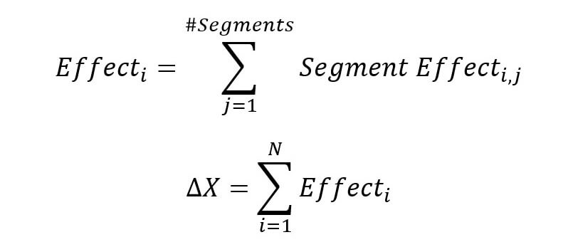
Following this approach would yield the updated formulas for variance analysis:

In practical steps, this hybrid approach would entail the following steps:
- Identify the relevant variables that can explain your metric (multiplication)
- Price, Quantity, Volume, Concentration, Currency, etc.
- Determine the relevant level of granularity for each business parameter (addition):
- Variable 1 (product): product -> model -> size -> edition
- Variable 2 (geography): region -> country -> city
- The cartesian product of the variables in step 2 will yield all the relevant possible combinations:
- Each combination is a segment (ex: small TVs sold in Utah)
- Compute your effects (price, quantity, currency…) at the segment level
- Aggregate your “atomic” segment effects to the desired macro level:
- Per effect, per country, per size, per color etc.
Conclusion
Before I conclude, I would like to thank you for reading this far.
I hope you got something useful out of this short post.
The idea can be generalized to other areas of finance and performance evaluation.
As a reimnder, don’t forget to weigh the pros and cons when determining the relevant level of granularity.
Stay tuned for the next posts in this variance analysis series.
