
Have you ever wondered if you could explain the change in a weighted average cost as a function of unit value changes instead of the usual approximations based on the total cost change?
What is this about?
In the first post of the Variance Analysis series, we went over the importance of increasing the “resolution” of our variance analysis to make more accurate business decisions that reflect the real financial picture of a given company.
In this second post, we will see how to expand the scope of variance analysis to explore the same financial data from a different point of view and hopefully derive a more holistic understanding of reality, leading us to more effective decisions.
Quick review
If you have not yet read the first installment of the Variance Analysis series, I strongly advise you to do so, in order to follow this post.
Follow this link to read the first post.
For the sake of review, let us go through a few formulas covered in the first post:
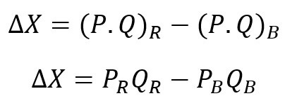
These formulas are essentially different ways to represent and explain the total gap in our metric (referred to throughout the article as price or cost).
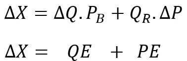
We also introduced an updated version of theses formulas that is more accurate:
Budget Variance Gymnastics
With the review out of the way, we can move on to the fun part.
Our first goal is to explain the change in average cost of a given segment.
A segment can be any business combination of interest (ex: white cars sold on February in Angola).
How should we go about it?
Well, fortunately we already have a formula that does a decent job.
It’s the basic variance analysis formula:
It just needs a little twist.
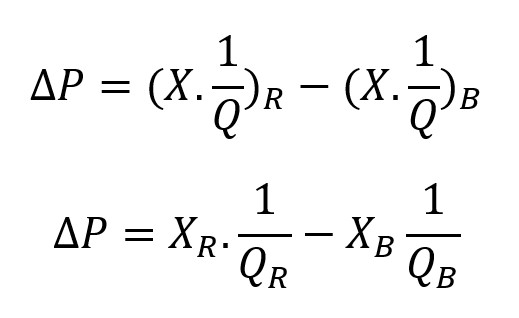
We will replace the metric X with its average (average price in our example):

The gap formula then becomes:
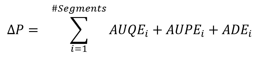
The basic variance analysis formula can then be expressed as follows :
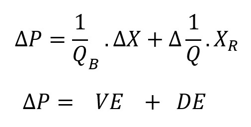
- Delta P: Price gap
- VE: Value Effect
- DE: Dilution Effect
We will go over each portion of the formula.
The value effect reflects the effect the increase of the total metric has on the average value of the initial quantity.
The problem is that the new average price is not relative to the initial quantity but rather relative to the new one.
This observation introduces the role of the dilution effect: a factor correcting the value effect to account for the difference in denominators.
You will notice that these effects do not explain the change in price from an endogenous angle (root causes such as inflation, productivity etc.).
It just describes the algebra through which the average price is formed.
The Value Effect Looks Familiar
The value effect is just the metric gap divided by the initial quantity:
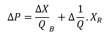
It follows that we can further expand it to account for our old friends from the first post, the total quantity effect and the total price effect:
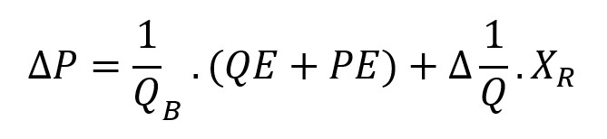
Ultimately, the change in the price can be expressed as the sum of 3 effects:

- UQE: Unit Quantity Effect
- UPE: Unit Price Effect
- DE: Dilution Effect
It is important to note that while the QE and PE effects do not overlap (explain independently one from the other), the dilution effect is affected by both changes in quantity and prices.
Despite this shortcoming, it is still important as it is the correction factor needed to obtain the average price.
Sounds like Regular Budget Variance with Extra Steps
I know, but please bear with me.
We reached our first goal of explaining a change in the average price of a segment.
We identified 3 effects and were able to quantify each one of them.
It is still of limited interest, because it is at the segment level.
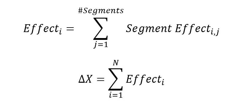
It becomes orders of magnitude more interesting once we combine it with the expanded variance analysis formula introduced in the first post:
This combination serves three purposes:
- More accurate quantification of the price and quantity effects;
- This formula aggregates effects at the segment level, introducing factors to explain more endogenously the changes in the total metric (business variables such as model, time, geography, demographics etc.);
- Introduces the aggregation of the dilution effect at the segment level.
Sounds good! How do we do it then?
We cannot directly sum the individual effects at the segment level.
The result would be skewed as we are considering the change in a weighted average.
Both the scale and the weights of each segment change and affect our result.
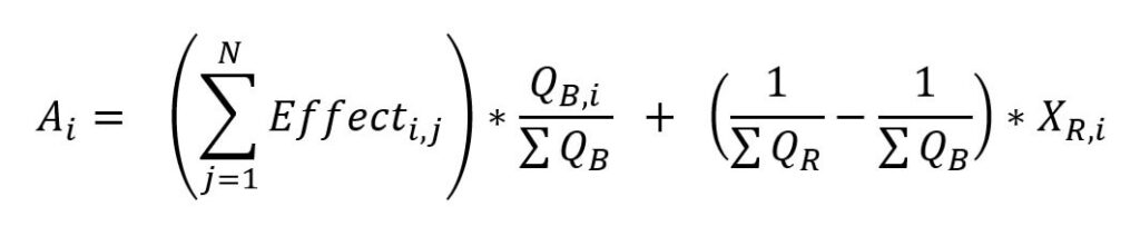
We need to adjust each segment effect with the right factors:
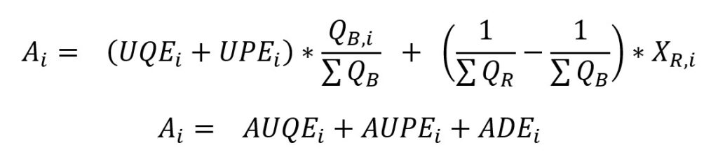
- Ai: Contribution of segment i to the change in the average price of the total of all segments
- AUQEi: Adjusted unit quantity effect of segment i
- AUPEi: Adjusted unit price effect of segment i
- ADEi: Adjusted dilution effect of segment i
UQE and UPE together represent the change in the total metric for segment i (what we referred to earlier as Value Effect, but at the segment level).
They are simply adjusted with the initial quantity corresponding to their segment.
The tricky part is adjusted by using the aggregate quantities instead of the segment quantities.
The adjustment formulas can even be expanded to take into accounts N effects (see first post):
The end result would be this little gem:
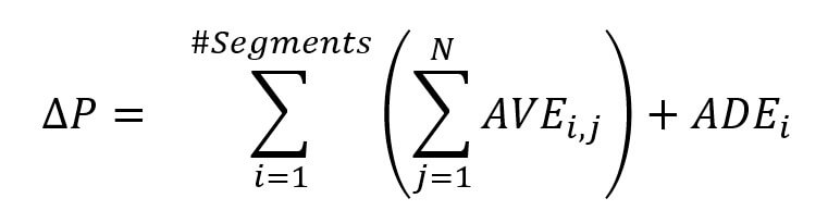
We will see in the next section that there is a more intuitive way to visualize this formula.
Case Study: Unit for Total and Total for Unit
The following case study can be downloaded if you want to have the formulas ready-made.
Download the Excel file here:
Following the bankruptcy of our Metaverse Land company (see first post), we decided to stick to a no-name company selling 4 products (A, B, C and D).
We are evaluating the inventories of the company to see how they changed from the end of Period 1 to the end of Period 2.
In this case, Period 1 will serve as “budget” or reference in our analysis.
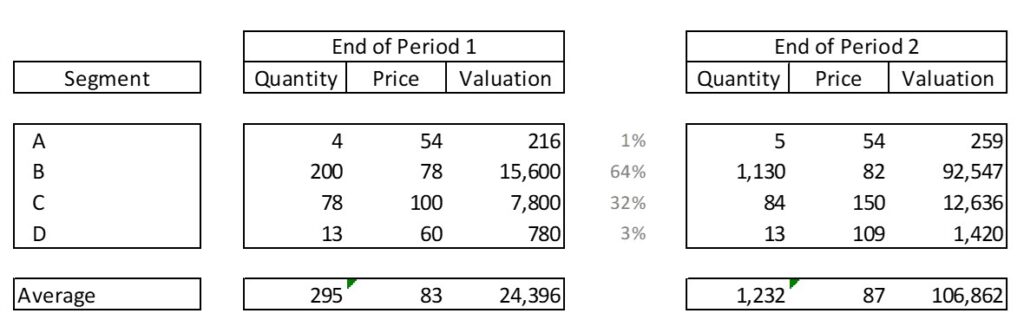
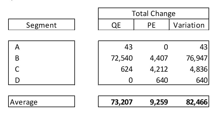
Next up is the total change in inventories as well as the different effects computed with the updated budget variance analysis formula:
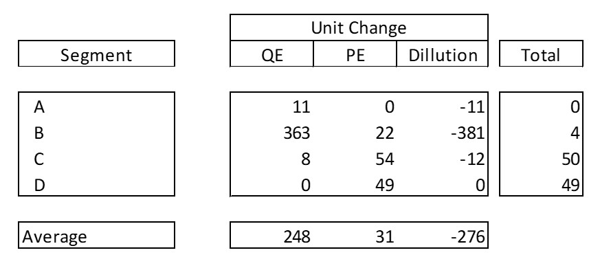
We then compute the unit effects for each segment:
Finally, we apply the last formula we covered to compute the contributions of each effect and segment to the total change in the weighted average value of the inventories:
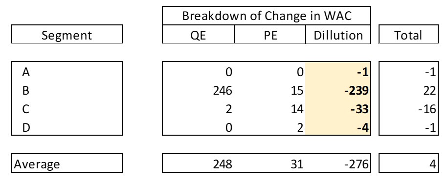
This matrix is the more intuitive way to visualize the formula as mentioned earlier.
We can tell the following elements by using the matrix:
- While all prices and quantities increased or stayed the same (all PEs and QEs are positive), the segments did not all contribute positively to the total average;
- If we apply the same growth rates to all segments for prices and quantities, the segments still do not contribute evenly to the total average;
- As the inventory mix changes, some segments increase in percentage of the total inventory valuation and others decrease (all changes must add up to 0);
- Both the initial composition and the change undergone in the mix affect the way segment effects impact the total average.
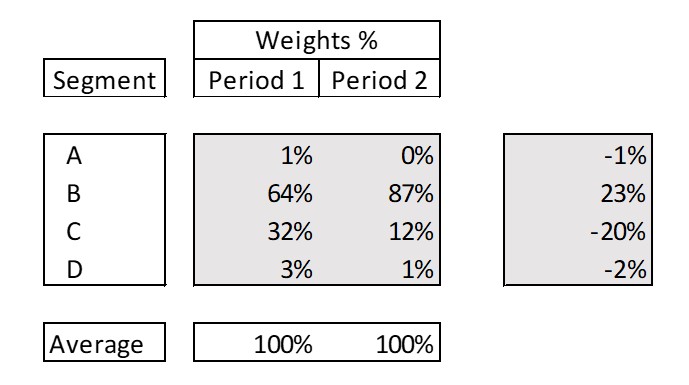
We can confirm our observations by computing the weights of each segment in terms of valuation:
Conclusion
I hope you found this article informative and useful.
The concepts outlined in this post may not be as practical as regular variance analysis but they fill a dark spot in the visual field of the financial analyst.
Frequently, changes in averages are attributed to vague causes such as changes in the volume and timing of cost inputs for lack of a better tool.
The emphasis is also usually placed on endogenous explaining factors.
The formulas shown here allow us to quantify the impact of the algebraic nature of the methods used to compute average costs.
The best approach would be a combination of both: endogenous factors explaining the changes at the segment level (input inflation, loss of productivity etc.) and the exogenous approach quantifying the impact of the changing mix.
It goes beyond FP&A or controllership; it can be used in any setting with averages and for any purpose.
To conclude, I would like to thank you for reading and please don’t hesitate to reach out as your feedback would be very much appreciated.